Introduction

We were given the task of creating a musical instrument with some sort of haptic feedback for the user. We first did individual design proposals and were organized into groups based on our ideas in those proposals. Based on our group's proposals, and one member's familiarity with acoustic guitars, we decided that our electronic instrument would be heavily inspired by a six-string acoustic guitar. In our group we found strengths especially in Arduino programming and MIDI/pd communication, and decided to use these as hardware and synthesizer.


The main components that we wanted to create was strumming of the "strings", creating different notes based on the string's position in the frets, and add light and vibrations to correspond with the note being played.

The members of our group are:

Kevin Melotti

Sean Murphy

Lisa Perez

Body Structure, Fret Sensing, and PD code

1) Body Structure

We first considered a minimalist shape, maintaining only the necessary contact points of an acoustic guitar. See an example of this in the Yamaha SVC-210 electric cello -->



However, after further consideration, much of an acoustic guitar is a contact point, and for simpler construction and electronic packaging we went with a traditional shape.

We wanted to keep the body fabrication simple. The guitar body is lasercut from 4mm wood, to create front and back sides. The two sides are joined with standoffs, and the electronics are attached by velcro to reduce necessary hardware. The only complication was the maximum size of the blanks which fit in the lasercutter, which forced us to cut the guitar from four parts instead of three.
We are pleased with the final shape and durability. It's blue paint, block M and recognizeable shape drew people to it at the expo, and it's structure was robust enough to survive with no damage.

2) Fret Sensing Concept

One of the key features of our instrument is its expressive range. We desired to keep all the note range and capability of an acoustic guitar as a baseline functionality. In order to sense each possible fret position of each six strings, we needed to be able to sense 6x24 positions independantly of each other. However, in a real guitar, only 6 positions are needed at a time, which is each string at the lowest fret fingered. Instead of attempting to assemble 144 sensors, we instead built the 24 frets to each carry a unique voltage, and then use the six metal strings themselves to close the circuit to the arduino analog in ports. The guitar neck is a giant voltage devider, and the strings pick off the voltage when applied to a fret. Otherwise the strings are pulled down to ground. As the analog in ports draw little current, the voltage devider sees very little change in Vout when the string 'load' is applied, and all strings can be fingered with reliable results.
In practice, it is difficult to establish a good connection between the strings and the frets, and while possible, each string must be carefully fingered to acheive the desired chord.

3) Pd code
We chose to produce MIDI output from the guitar, and use Pd as a synthesizer. We decided to do this because we were confident we could produce a satisfying output in this manner. MIDI was only used as a communication standard, as we were creating the Pd patch from scratch, we did not use standard MIDI commands.
Basic MIDI includes note-on and note-off commands, and the simplest synthesizer will produce a pure tone of the commanded note at the commanded volume until the note-off command. A guitar is much different, with each string acting largely independantly of each other (ignoring the excitation one string may cause on another) and each sounding at the same time as the others and with their own overtones. Additionally, ignoring fret-work (hammer on/off, bending) the strings work on their own after initial impulse excitation, dynamic volume is not necessary. The structure of the Pd patch reflects the impulse input control, and independance of each string.
The Arduino sends the note and volume when the string is triggered. Pd receives the command and acts on the trigger, sending the command to the appropriate 'string' subsystem, which sounds the note and calculated overtones with the triggered ASDR envelope ("Attach, Sustain, Decay, Release"), tuned according to our observed acoustic guitar behavior. Each of the six strings has its corrosponding subsystem, which follow their own envelopes. This allows chords when multiple subsystems are sounding at the same time, triggered quickly in succession in a natural strumming motion.
There is also capability to pitch bend the final total output of the patch. If there is a continuous sending of MIDI information above the string information range this will work on the pitch shift.
The sound generation is simple: a phasor is constructed at the main frequency and at smaller magnitudes at the first two overtones. The ASDR envelope has an aggressive attack to emulate the aggressive attach in a string pluck. While effective in creating a pleasant and musical tone, there is further room to acheive a more accurate acoustic guitar sound, if desired.

Pd guitar front-end. Note-in sends information to correct 'string' or pitch bending


Example 'string'. Each string has unique asdr envelope


Borrowed ASDR envelope patch

Main Body's Arduino

Strumming

While we were brainstorming we thought of ideas to create a feeling of a pick being forced over multiple strings. To accomplish this task we used a linear actuator with an attached potentiometer to create the haptic environment. Specifically we used the motorized fader provided by class. We had the idea of creating a virtual spring that would give way once the "string" was passed. The force curve would look similar to a ramp function. To create this kind of feel we needed to know the position and direction of the velocity from the potentiometer. We used an op amp circuit in order to find the velocity direction. The circuit diagram below shows how we found the position and velocity from the potentiometer on the fader motor.

Once we had the position and velocity for the Arduino we used an H-Bridge to control the motor of the fader. We compared the current position to the position of the virtual spring and as the current position came closer to the virtual spring the force would increase. Once the position past the string the force would let up. We used the velocity to determine which direction the fader is moving so that we can get the string feeling regardless of which direction the user was strumming. The code for this can be seen in the Appendix Post under older posts.

Detecting and Sending a Note


To determine when a note was being played we monitored the position of the motorized fader. When it crossed a particular position (designated as a "string")we proceeded to send a note and send a signal to the other Arduino. We used a MIDI to communicate with the computer using the connection diagram found in this tutorial. With that we sent a signal to the computer. The signal consisted of three bytes of data (channel, note, volume). We used channel 1 for all communications. The note was determined by the particular string being strummed and which fret that string was pressed into. So for string 1 we sent a number between 0 and 15 (we had 15 frets and open), for string 2 we sent a number between 16 and 30, and so on up to 6 strings. For the volume we sent a byte between 70 and 110. The particular value was determined by an accelerometer located in the guitar's body. We used an axis aligned with the neck of the guitar and used gravity to determine the tilt of the guitar. We then sent a larger value for the volume when the neck was tilted up and a smaller value when the neck was tilted down. The code for this can be seen below.

Communication to the Other Arduino


Another task that the main body's Arduino had was to send a signal to the other Arduino signaling that a string had been strummed. This is required to allow the other Arduino control the lights and pager motors at the head of the guitar. To do this we were going to send the signal that corresponds to the volume of the guitar when a string is strummed. We went about this by using an analog write to a pin that the other Arduino would read. But since an analog write on the Arduino board produces a PWM and reads a specific value we were only getting 0 or 5 volts reading. To overcome this we put the signal through a low pass filter to smoother the signal out.

To create a low pass filter we had a signal go through a 5.6 kOhm resistor then at this node we had a 1 microFarad capacitor connected to ground and a wire going to the other Arduino. The code that we used to communicate can be seen in the Appendix Post in older posts

Head of the Guitar

The head of the guitar is where the vibration of the body and the visual feedback are controlled. This part of the design consists of an Arduino Duemilanove controller, 2 pager motors (vibration), and 6 LEDs (visual feedback). The vibration and visual feedback are discussed separately below.

Vibration: To give the feeling that a real acoustic guitar gives when its strings are plucked, we decided to include 2 pager motors that spun at a certain speed at the neck of the guitar as soon as a one of the virtual strings was plucked. The certain speed was determined by what the volume was – the higher the volume, the higher the speed. To get the volume data, we ran a line from an Arduino Mega Analog Out pin to the Duemilanove’s Analog In pin. We mapped that data to a full PWM range, which created 2 signals that controlled both motors.

As long as the virtual strings were not being plucked, the speed of the motors would attenuate over a given amount of time to simulate the dying down of the vibrations. We based this given amount of time (about 15 seconds for loud plucks) on tests that we did with a real acoustic guitar.

Visual Feedback: We decided to add an element of “Star Power” in our design by creating a light-up block M that had 3 levels of lighting that would react to the volume in a manner similar to the pager motors. To do this, we mapped the same volume data to PWM ranges, which created 3 signals that controlled 3 sets of 2 LEDs in parallel.

As long as the virtual strings were not being plucked, the lighting would attenuate over a given amount of time. The top tier of LEDs was mapped to the smallest PWM range, so it started to dim first. The second tier was mapped to the middle range, so they started to dim about a second after the top tier. The third tier was mapped to the highest range, so it dimmed last.

The code for this can be found in the Appendix section under older posts.

Layout:

Assembly and Tuning

Upon assembly we found some areas did not go together as smoothly as planned. The biggest problem was the strings and accelerometer input into the lower arduino; the values read did not make sense, and did not match voltmeter readings made on the inputs directly. This was finally resolved when we found the Arduino v.17 program to have a bug in the computer software side. When this was resolved, the readings cleared up. Other more minor issues in were:

a) The body structure was not sufficiently reinforced at the body-neck connection, and the neck had become quite heavy with the upper arduino and voltage-devider fret board. This was fixed with a neck-body reinforcement made of balsa, wood glue and through-bolts.

b) The strings were not sufficiently 'pulled-down' and an open fingering did not give consistant results. Resolved with different pulled-down resistor values

c) The accelerometer was not functioning properly. This was cleared up when the datasheet was examined and the part was found to function on 3V instead of the 5V we were running it at.

A video of our final product can be seen below:

Product at MechaMusicTronics Event

We took our design to MechaMusicTronics in the Duderstadt Gallery. We were slightly worried about how it would go over with the crowd, especially since it wasn't tuned perfectly. However, guitar players and non-guitar players alike definitely engaged with the design, from the fader motor's ability to simulate plucking a string, to the voltage divider frets, to the vibrations of the guitar, to the light-up M.

Here are some pictures from Monday:

Future Functionality and Design Revisions

Now that the baseline guitar is constructed, future work can add novel functionality and expand the expressive range of the instrument. First, pitch bending may be implemented - the accelerometer hardware and pd code is in place, just the Arduino code needs to be adjusted, and then overall pitch could be altered by tilting the guitar.


Another idea we had was a built-in sequencer. The arduino memory could be used to store a section of playing, perhaps commanded by another external button, and then that could be played on command, or looped under continued playing. Different expansions on this same idea: the Arduino could loop just the fingering or just the picking, allowing the player to concentrate on the other to produce more complex music more easily.


To expand the 'acoustic guitar' functionality, the arduino could carry multiple tuning maps onboard, to be selected by the player to automatically assign the fretboard different tuning, or a virtual capo.

Appendix

Appendix A:

Code for Main Body's Arduino

const int string[] = {5,4,3,2,1,10};//10,1,2,3,4,5};
int stringval[6];
int pos[6];
const int position = 6;
int dir = 12;
int pwm = 13;
int direct = 7;
int i = 0, q = 0;
int j = 0;
float k = 1;
int dir1 = 0;
int vol = 0, xval=500, var=0;
const int commout = 3, xaxis=8, yaxis=9;
int pitch = (255-146)/2;

void setup() {

Serial.begin(31250);
pinMode(direct,INPUT);
pinMode(pwm,OUTPUT);
pinMode(dir,OUTPUT);
}

void comm(int x, int a, int y, int z, int b){
if (x <> 50)
{
//Sends a MIDI signal and the other Arduino a signal
if ((x-a+3 > z-a-3)) {
noteOn(0x90,16*(z/(1023/7)-1)+stringval[z/(1023/7)-1],b);
analogWrite(commout,map(vol,70,110,0,150));
delay(15);
}
else if (a-x+3 > a-(z-1023/7)-3) {
noteOn(0x90,16*(z/(1023/7)-2)+stringval[z/(1023/7)-2],b);
analogWrite(commout,map(vol,70,110,0,150));
delay(15);
}
//Creates a feedback for the user (virtual spring)
if (y <495){>525)
{
if (x>z-1023/14+15) {
analogWrite(pwm,0);
} else {
analogWrite(pwm,abs(z-x)*k);
analogWrite(dir, 255);
}
}
}
else {
analogWrite(pwm,1);
}
}




void noteOn(byte cmd, byte data1, byte data2) {
Serial.print(cmd, BYTE);
Serial.print(data1, BYTE);
Serial.print(data2, BYTE);
// Serial.print("cmd ");
// Serial.print(cmd, HEX);
// Serial.print(" data1 ");
// Serial.print(data1, HEX);
// Serial.print(" vol ");
// Serial.println(data2, HEX);
}




void loop() {
//reads the value of each string to determine fret position
i=i+1;
q=q+1;
if (i==6) {
i=0;
}
stringval[i]=map(analogRead(string[i]),-14,970,0,15);///(1023/15);


//reads the position of the fader and direction it's traveling
pos[i] = analogRead(position);
dir1 = analogRead(7);
vol = map(analogRead(xaxis),295,400,110,70);
if (i==0) { j = 5; }
else { j = i-1; }

//Sends the position, past position, direction, string it's closet to, and the volumn to the

//commuication function
if (pos[i] <= 1023/7) { comm(pos[i],pos[j],dir1,1023/7,vol); }else if (pos[i] <= 2*1023/7) { comm(pos[i],pos[j],dir1,2*1023/7,vol); } else if (pos[i] <= 3*1023/7) { comm(pos[i],pos[j],dir1,3*1023/7,vol); } else if (pos[i] <= 4*1023/7) { comm(pos[i],pos[j],dir1,4*1023/7,vol); } else if (pos[i] <= 5*1023/7) { comm(pos[i],pos[j],dir1,5*1023/7,vol); } else if (pos[i] <= 6*1023/7) { comm(pos[i],pos[j],dir1,6*1023/7,vol); } else { comm(pos[i],pos[j],dir1,7*1023/7,vol); } //sends the other Arduino a constant flat line analogWrite(commout,1); }





Code for Arduino at Head of Guitar:
int i = 0; int var = 0; int varLed1 = 0; int varLed2 = 0; int varLed3 = 0; int myData = 0;

int ledPin1 = 3; int ledPin2 = 5; int ledPin3 = 6; int motorPin1 = 11; int motorPin2 = 10; int volInput = 1;

void setup(){
Serial.begin(38400);
pinMode(motorPin1, OUTPUT);
pinMode(motorPin2, OUTPUT);
}

void loop() {
myData = analogRead(volInput);
Serial.println(myData);
if(myData > 50) { i = 0;}
var = map(myData, 0, 900, 0, 255);
varLed1 = map(myData, 0, 900, 0, 255);
varLed2 = map(myData, 0, 900, 0, 175);
varLed3 = map(myData, 0, 900, 0, 125);
if(i <255){
analogWrite(motorPin1, var-i);
analogWrite(motorPin2, var-i);
analogWrite(ledPin1, varLed1-i);
if(i <125){
analogWrite(ledPin2, varLed2-i);
analogWrite(ledPin3, varLed3-i);
}
else if(i <175){
analogWrite(ledPin2, varLed2-i);
analogWrite(ledPin3, 1);
}
else if(i <255){
analogWrite(ledPin2, 1);
analogWrite(ledPin3, 1);
}
delay(5);
i = i + 1;
}
else{
analogWrite(motorPin1, 1);
analogWrite(motorPin2, 1);
analogWrite(ledPin1, 1);
analogWrite(ledPin2, 1);
analogWrite(ledPin3, 1);
}
}

Schematic of the system in interest

For our system we decided to use the motorized fader. We will be using this in our project as a way to mimic virtual guitar strings. A rough schematic can be seen in the image below.

The way the motorized fader works is by a rotary motor driving a belt that drives a slider. The slider has a potentiometer that determines the position of the fader. We will be using the position in this lab and in our future project.

The key parts that we are interested in is the voltage required by the motor to produce the desire feedback force at F_H and the position of the fader. The desired feedback force will be determined by the position of the fader. Therefore we wished to find the transfer function relating the input voltage to the position of the fader in this lab. The circuit setup with the physical motorized fader can be seen in the image below.

Lab 6 Overview

For the lab, we used a fader motor, as it is the component that we will be using to haptically simulate the strings of our virtual guitar. Given that we had not previously performed a system identification for this fader motor, we cannot provide a comparison with the experimental frequency response plot.

Though we cannot provide a direct comparison, we can make judgments based on our observation of the motor behavior and compare our experimental plot with those. For example, as is apparent by the fact that a sound comes from the motor when we run it, there is metal on metal contact, which leads to a great deal of friction in the system. Because of this friction, system identification should return an overdamped system. Overdamping was definitely the case for the lab.

For future purposes, we plan to perform a system identification by loading a variety of masses on the fader motor so that, in the long run, we can better understand the system instead of just making judgments and best achieve the behaviors we want for our virtual guitar.

Lab 6 Overview

1) Compare theoretical and experimental frequency response plots by placing traces on the same axes. Show these for your low-pass filter:

We built an RC low-pass filter with a 430 Ohm resistor and 2.2E-4 Farad capacitor. This should produce a 1st order system with a w_cutoff of 10.6 Hz. Below is our input and output plotted, which was submitted to TFestimate and produced the given Bode plots:

RC, Arduino, Matlab input/output
Blue: input white noise, Red: RC voltage output

Bode from TFestimate
Notice w_c on magnitude plot

Trouble w/Phase response....
As far as the phase response goes, we did not get anywhere close to good results. This was much in part due to the delays in the Arduino and MATLAB.

day 4 - Arduino Success

Today we successfully characterized both our linear motor and a simple low-pass RC filter with the Arduino, connected by serial port to matlab.

Picking up where we left off yesterday, we quickly sorted the programming trouble and successfully stored Matlab-generated white noise data to the Arduino. Even with only streaming the data one direction, from the arduino to matlab, and shortening the transmit to a single byte, we were only able to acheive 60Hz.

Next step was to store the output data to the arduino as well, and then transmit it after the motion loop was finished. We had been hesitant to employ this, as it would require timekeeping on the arduino side, which in our group members' previous experience slowed the arduino down greatly, and we were also unsure about the arduino memory capacity. However, we implemented and ran it, and were pleasantly surprised to find the loop could deliver a data point every millisecond, resulting in a 1000Hz sampling frequency. Also, the arduino had no trouble storing up to 800 samples, each with white noise command, position, and time.

For our highly damped linear motor, the 1000Hz sample time was appropriate. Keeping that constraint in mind, we assembled a low pass filter with a relatively low critical frequency for successful validation.

Day 3 - Arduino-to-matlab communication

Today we spent a couple hours working on getting the arduino and matlab to communicate over the serial port, and then to run the white noise command and receive position output at an acceptable frequency. We started by examining Team 7's sequencer code from the previous lab, which streamed data to matlab, and waited for matlab data back to respond.

After sorting the code we did set up streaming white noise, and returned streaming position, using Matlab to time stamp the data with the built-in tic and toc function. Unfortunately, we could only push the data to 10-20Hz, and it became unreliable at higher frequencies.

To increase frequency, we went to transmit and store the white noise data to the Arduino. We ran into programming trouble getting the data to store correctly, and called it quits.

Day 2 - Lab plan and project-pertinent plant

Today we met to review the lab assignment and choose our plan to obtain data for TFestimate. We chose to use a linear motor with built in potentiometer as used in Lab 5 as an actuator in our final project, and therefore will find the transfer function from H-Bridge command to linear potentiometer position output. We built the circuit and mechanism for this. We chose to re-use some code from a member's lab 5 project for arduino-to-matlab communication, and broke off the meeting while waiting to get the code in hand.

Lab 6 - Day 1, sysidexample.m Exploration

Team members...
Kevin Melotti
Sean Murphy
Lisa Perez


Today we got a handle on the sysidexample.m matlab file, and the tfestimate function. Below is a plot of a second-order system simulated and run through TFestimate, green circles are analytical results, blue line is from TFestimate in all plots:


We explored changing sample frequency and period. As expected, reduced sample frequency led to undefined high frequency behavior prediction, and reduced sample period limits low frequency behavior. See plots below:

Low (100Hz) Frequency

Short Period:

Lab 4 - Our process, in detail

Method
In the previous lab, we were using a Hall-effect sensor to measure the position of the pendulum. The sensor produced voltage in the range of 2.0V to 3.0 V, which is read by the Arduino's analog reading as a value between 495 and 540. With this range, the position only has 45 data points and this resolution is not sufficient to reproduce a good virtual spring and damping. When we use the sensor readings to determine the speed of the pendulum, it often takes into account the random noise from the Hall-effect sensor and since the resolution was poor, the PWM output tended to be large. This resulted in a lot of stability problem in our control.

In this lab, we used OP Amp to amplify the voltage range so that the output voltage came in the voltage range of 0V to 5.0V, which enabled us to use the full extent of the Arduino's analog input range. Below is the circuit diagram of the OP Amp we used in this lab.

We set the positive terminal to be 2.5V so that the neutral position of the output voltage from the OP Amp to be 2.5V. We choose this value to match the middle output of the Hall-effect sensor. The resistors in the negative terminal are used to amplify the ±0.5V voltage range from the Hall-effect into ±2.5V so that the voltage output range from the OP Amp has a range of 2.5V ±2.5V or 0V to 5V. Since this is an inverting OP Amp, the gain is reversed so that 2.5V±0.5V range translated into 2.5V±(-2.5V) range for the output from the OP Amp.

Theoretically, we should get this range of 0V to 5.0V, but the middle point of the Hall-effect sensor turned out to be not exactly on 2.5V, so the actual output voltage range from the OP Amp came out to be between 0V and 4.0V. This is still a huge increase in voltage range, and the analog reading from the Arduino read values between 0 and 827. The new range has more than 800 data points, which is approximately 20 times as large as the original.

With the new resolution, we can try the previous lab's code to test the virtual spring and damping and see if there is any improvement in the controls.





With the new resolution from the OP Amp, we edited the previous lab's code to adjust with the new analog reading values. We decided to try the proportional control first. With the new resolution, the movement of the pendulum looked more fluid compared to the old resolution and the motion is more "spring-like". However, there are still some noises inside the reading of roughly ±30 data points, which is large because it is also got amplified by the OP Amp. When we moved into the derivative control, there was no significant improvement compared to the previous lab's. Large noises still present and instability still occurred.

You can see the proportional and derivative control at work in the video below.

Once we accomplished this, we moved to programming the Arduino to send amplified analog data from the hall effect sensor to the PD interface. We downloaded Arduino2PD patches available on programmer websites, and altered them to meet our needs, as there were no functions dedicated to actually playing the notes in the original patches.

Results
PD programming: We ended up with the program below (Note the change in port number and speed ("comport 19 38400") and the addition of five function blocks to play a note).

The first five analog in number boxes do not apply here. They would only apply if we were using multiple sensors with analog outputs. The number that we want to pay attention to is the analog in 5 number, which is the exact number that the hall effect sensor would have returned even if placed in circuit with solely the Arduino.

Discussion
Virtual environment testing: OP amp does help by increasing the resolution of the output, but does not help with reducing the noise, which was the major problem for the derivative control.

PD programming: We subtracted 500 and multiplied the result by 1.5 so that we could (a) only play notes if the armature was displaced from equilibrium and (b) get the largest range possible. If we multiplied by more than 1.5, the range would be the same but within a smaller domain. If we multiplied by less than 1.5, on the other hand, the range would not reach the highest note possible, even when armature was fully displaced. The value of 1.5 gave us the optimal performance for our set-up.

After that was completed, it was easy for us to integrate the virtual spring with tuned values from the first part of this lab. As previously mentioned in the "Accomplishments" section of the last blog post, we ended up with an instrument that played higher notes and gave higher feedback forces as the armature's displacement from center increased.

Lab 4 - Working with MIDI

The Team:
Lisa Perez
Amit Ranjan
Andrew Rohr
Eric Sihite

Our Goals for This Lab:
During the first part of this lab, we aimed to minimize quantization error by switching out our hall effect sensor from the last lab with a more sensitive hall effect sensor and maximizing the output range by the sensor by putting it in circuit with on op amp. After minimizing error, we aimed to obtain a velocity reading by differentiating the position signal with another op amp. We planned to integrate the improved settings with our virtual environments from the last lab.

The second part of lab entailed integrating a haptic environment of our motor with a MIDI interface to create a haptic instrument. For this, we aimed to understand how to send information from the Arduino to PD, our software synthesis interface, and what to program in PD to be able to get a noise and force feedback just from manipulating the motor armature.

What We Accomplished:
We were excited to use the new hall effect sensors to obtain better settings. However, shortly after soldering the terminals, one of the terminals broke, and we were not able to solder it back on. Instead, we obtained one of the older hall effect sensors and completely our work with that. We were able to get a larger output range from the op amp, with serial ouput ranging from 0 to 815 (in contrast to the approx. 500-600 range).

Even though the hall effect sensor was the same model that we had used in the last lab, we had to tweak the programming slightly to account for a difference in behavior. Once we did this, however, we were able to resimulate our virtual environments.

After we did this, we did a search on how to integrate the Arduino with PD, an interface that allows software synthesis. We learned that we could download preexisting patches for both the Arduino and PD, and altered these patches for our needs, such that the information from the hall effect sensor would transfer correctly from the Arduino to the PD interface, and consequently to the speakers.

After a few hours of looking at programming in Arduino and PD, we were able to get tones from the speakers by moving the armature back and forth. We tweaked the numbers to make it so that the armature only played if displaced from center, with higher notes being further away from center. We included a virtual spring so that the users would feel more force further away from center (and thus with a higher note).

Lab 3 - Virtual Environment Code (Virtual Spring-Mass)

////////////////////////////////////////////////////////////////////////
// Declare Pin Assignments
////////////////////////////////////////////////////////////////////////

const int currentSensorPin = 1;
const int positionSensorPin = 7;
const int dirMotorPin = 22;
const int pwmMotorPin = 9;
const int ledPin = 13;
const int speakerPin = 10;

////////////////////////////////////////////////////////////////////////
// Declare Variables
////////////////////////////////////////////////////////////////////////

int sensorValue = 0; // the sensor value
int sensorMin = 1023; // minimum sensor value [Position Sensor]
int sensorMax = 0; // maximum sensor value [Position Sensor]

int t_step = 5; // Delay Between Control Loops (microseconds)
int freq = 2000; // PWM Frequency (Hz)

double thetaMin = -18.0; // Minimum Position Angle
double thetaMax = 18.0; // Maximum Position Angle

int position_sign;
double pwmMin = 0.00; // Minimum Duty Cycle
double pwmMax = 1.00; // Maximum Duty Cycle
double A;
double B;

double K_m = 0.0153261; // Motor Torque Constant
double pi = 3.1415;
double delay_ = 0.001; //delay in seconds

////////////////////////////////////////////////////////////////////////
// VIRTUAL MASS-SPRING SYSTEM
////////////////////////////////////////////////////////////////////////

double xBlock0 = 0.;//0.05;
double xBlock = 0.05;
double vBlock = 0.;
double aBlock = 0.;
double mBlock = 10.;
double rLever = 0.02;
double kSpring = 100.;
double dt = 0.05;

////////////////////////////////////////////////////////////////////////
// Setup Function
////////////////////////////////////////////////////////////////////////

void setup() {

// Set Input Pins

pinMode(currentSensorPin, INPUT);
pinMode(positionSensorPin, INPUT);

// Set Output Pins

pinMode(dirMotorPin, OUTPUT);
pinMode(pwmMotorPin, OUTPUT);
pinMode(ledPin, OUTPUT);
pinMode(speakerPin, OUTPUT);

// Signal Beginning of Calibration
digitalWrite(ledPin, HIGH);

// Calibrate during First 10 Seconds
while (millis() < sensorvalue =" analogRead(positionSensorPin);"> sensorMax) {sensorMax = sensorValue;}

// record the minimum sensor value
if (sensorValue < sensorMin) {sensorMin = sensorValue;}

}

// Signal End of Calibration
digitalWrite(ledPin, LOW);

// Initialize Serial Communication Connection
Serial.begin(9600);

}

////////////////////////////////////////////////////////////////////////
// Loop Function
////////////////////////////////////////////////////////////////////////

void loop() {

double theta;
double dutyCycle = pwmMin;
double current;
double currentDesired;
double torqueDesired;

// Read Position Sensor
sensorValue = analogRead(positionSensorPin);

// Find Angle Using Sensor Value
A = (thetaMax-thetaMin)/(sensorMax-sensorMin);
B = (-0.5*(thetaMax-thetaMin))-(sensorMin*A);

theta = (A*double(sensorValue))+B;

// Print Processed Value to Serial Terminal
// Serial.print(" Theta: ");
// Serial.println(theta);

double force;

// Calculate Desired Torque
force = -1*kSpring*(xBlock - rLever*sin(theta*pi/180.));
aBlock = force/mBlock;

vBlock += aBlock*delay_;
xBlock += 0.5*aBlock*(delay_*delay_)+vBlock*delay_;

dutyCycle = force*rLever;

if (dutyCycle < 0) {position_sign = 0;}
else {position_sign = 1;}

// Use Limits on Duty Cycle
dutyCycle = constrain(abs(dutyCycle), pwmMin, pwmMax);

// Print dutyCycle to Serial Terminal
//Serial.println(dutyCycle);

// Set H-Bridge Direction
if (position_sign == 0) { digitalWrite(dirMotorPin, LOW); }
else { digitalWrite(dirMotorPin, HIGH); }

// Apply H-Bridge PWM Signal
dutyCycle = dutyCycle*255;
analogWrite(pwmMotorPin,int(dutyCycle));

delay(int(delay_*1000.));
}

Lab 3 - Virtual Environment Code (Virtual Damper)

////////////////////////////////////////////////////////////////////////
// Declare Pin Assignments
////////////////////////////////////////////////////////////////////////

const int currentSensorPin = 1;
const int positionSensorPin = 7;
const int dirMotorPin = 22;
const int pwmMotorPin = 9;
const int ledPin = 13;

////////////////////////////////////////////////////////////////////////
// Declare Variables
////////////////////////////////////////////////////////////////////////

int sensorValue = 0; // the sensor value
int sensorMin = 1023; // minimum sensor value [Position Sensor]
int sensorMax = 0; // maximum sensor value [Position Sensor]

double thetaMin = -18.0; // Minimum Position Angle
double thetaMax = 18.0; // Maximum Position Angle

int position_sign;
double pwmMin = 0.00; // Minimum Duty Cycle
double pwmMax = 1.00; // Maximum Duty Cycle
double A;
double B;

double K_m = 0.0153261; // Motor Torque Constant
double b = 0.0001;

double theta;
double dutyCycle;
double thetaOld = 0;

////////////////////////////////////////////////////////////////////////
// Setup Function
////////////////////////////////////////////////////////////////////////

void setup() {

// Set Input Pins

pinMode(currentSensorPin, INPUT);
pinMode(positionSensorPin, INPUT);

// Set Output Pins

pinMode(dirMotorPin, OUTPUT);
pinMode(pwmMotorPin, OUTPUT);
pinMode(ledPin, OUTPUT);

// Signal Beginning of Calibration
digitalWrite(ledPin, HIGH);

// Calibrate during First 10 Seconds
while (millis() < sensorvalue =" analogRead(positionSensorPin);"> sensorMax) {sensorMax = sensorValue;}

// record the minimum sensor value
if (sensorValue < sensorMin) {sensorMin = sensorValue;}

}

// Signal End of Calibration
digitalWrite(ledPin, LOW);

// Initialize Serial Communication Connection
Serial.begin(9600);

}

////////////////////////////////////////////////////////////////////////
// Loop Function
////////////////////////////////////////////////////////////////////////

void loop() {

// Read Position Sensor
sensorValue = analogRead(positionSensorPin);

// Find Angle Using Sensor Value
A = (thetaMax-thetaMin)/(sensorMax-sensorMin);
B = (-0.5*(thetaMax-thetaMin))-(sensorMin*A);

theta = (A*double(sensorValue))+B;

// Print Processed Value to Serial Terminal
// Serial.print(" Theta: ");
// Serial.println(theta);

if ((theta-thetaOld) < 0) {position_sign = 1;}
else {position_sign = 0;}

// Calculate Duty Cycle
dutyCycle = b*abs(theta-thetaOld)/(0.05);

thetaOld = theta;

// Use Limits on Duty Cycle
dutyCycle = constrain(dutyCycle, pwmMin, pwmMax);

// Print dutyCycle to Serial Terminal
// Serial.println(dutyCycle);

// Set H-Bridge Direction
if (position_sign == 1) { digitalWrite(dirMotorPin, LOW); }
else { digitalWrite(dirMotorPin, HIGH); }

// Apply H-Bridge PWM Signal
dutyCycle = dutyCycle*254;
analogWrite(pwmMotorPin,int(dutyCycle));

delay(50);

}

Lab 3 - Virtual Environment Code (Virtual Wall)

////////////////////////////////////////////////////////////////////////
// Declare Pin Assignments
////////////////////////////////////////////////////////////////////////

const int currentSensorPin = 1;
const int positionSensorPin = 7;
const int dirMotorPin = 22;
const int pwmMotorPin = 9;
const int ledPin = 13;
const int speakerPin = 10;

////////////////////////////////////////////////////////////////////////
// Declare Variables
////////////////////////////////////////////////////////////////////////

int sensorValue = 0; // the sensor value
int sensorMin = 1023; // minimum sensor value [Position Sensor]
int sensorMax = 0; // maximum sensor value [Position Sensor]

int t_step = 5; // Delay Between Control Loops (microseconds)
int freq = 2000; // PWM Frequency (Hz)

double thetaMin = -18.0; // Minimum Position Angle
double thetaMax = 18.0; // Maximum Position Angle
double thetaCenter = 0.0; // Center Position Angle
double K = 50;

int position_sign;
double pwmMin = 0.00; // Minimum Duty Cycle
double pwmMax = 1.00; // Maximum Duty Cycle
double A;
double B;

double K_m = 0.0153261; // Motor Torque Constant

////////////////////////////////////////////////////////////////////////
// Spring Force Calculation Function
////////////////////////////////////////////////////////////////////////

double torqueSpring(double theta, double thetaCenter, double K ) {

double torque;

if (abs(theta) > 5) {
torque = -K*(theta-5);
}
else {
torque = 0;
}

return torque;

}

////////////////////////////////////////////////////////////////////////
// Setup Function
////////////////////////////////////////////////////////////////////////

void setup() {

// Set Input Pins

pinMode(currentSensorPin, INPUT);
pinMode(positionSensorPin, INPUT);

// Set Output Pins

pinMode(dirMotorPin, OUTPUT);
pinMode(pwmMotorPin, OUTPUT);
pinMode(ledPin, OUTPUT);
pinMode(speakerPin, OUTPUT);

// Signal Beginning of Calibration
digitalWrite(ledPin, HIGH);

// Calibrate during First 10 Seconds
while (millis() < 10000) {

sensorValue = analogRead(positionSensorPin);

// record the maximum sensor value
if (sensorValue > sensorMax) {sensorMax = sensorValue;}

// record the minimum sensor value
if (sensorValue < sensorMin) {sensorMin = sensorValue;}

}

// Signal End of Calibration
digitalWrite(ledPin, LOW);

// Initialize Serial Communication Connection
Serial.begin(9600);

}

////////////////////////////////////////////////////////////////////////
// Loop Function
////////////////////////////////////////////////////////////////////////

void loop() {

double theta;
double dutyCycle = pwmMin;
double current;
double currentDesired;
double torqueDesired;

// Read Position Sensor
sensorValue = analogRead(positionSensorPin);

// Find Angle Using Sensor Value
A = (thetaMax-thetaMin)/(sensorMax-sensorMin);
B = (-0.5*(thetaMax-thetaMin))-(sensorMin*A);

theta = (A*double(sensorValue))+B;

// Print Processed Value to Serial Terminal
Serial.print(" Theta: ");
Serial.println(theta);

// Store Direction Information
if (theta < 0) { position_sign = 1; }
else { position_sign = 0; }

// Read Current Sensor
sensorValue = analogRead(currentSensorPin);

// Find Current Using Sensor Value
current = double(sensorValue)*(5/1023);

// Calculate Desired Torque
torqueDesired = torqueSpring(theta, thetaCenter, K );

// Calculate Desired Current
currentDesired = abs(torqueDesired/K_m);

// Print Current
// Serial.print(" Current: ");
// Serial.println(current);
// Serial.print(" Current Desired: ");
// Serial.println(currentDesired);

// Calculate Duty Cycle
double GAIN = 0.01;
dutyCycle = dutyCycle + GAIN*(currentDesired - current);

// Use Limits on Duty Cycle
dutyCycle = constrain(dutyCycle, pwmMin, pwmMax);

// Print dutyCycle to Serial Terminal
// Serial.println(dutyCycle);

// Set H-Bridge Direction
if (position_sign == 0) { digitalWrite(dirMotorPin, LOW); }
else { digitalWrite(dirMotorPin, HIGH); }

// Apply H-Bridge PWM Signal
dutyCycle = dutyCycle*255;
analogWrite(pwmMotorPin,int(dutyCycle));

}

Lab 3 - Virtual Environment Code (Virtual Spring)

////////////////////////////////////////////////////////////////////////
// Declare Pin Assignments
////////////////////////////////////////////////////////////////////////

const int currentSensorPin = 1;
const int positionSensorPin = 7;
const int dirMotorPin = 22;
const int pwmMotorPin = 9;
const int ledPin = 13;
const int speakerPin = 10;

////////////////////////////////////////////////////////////////////////
// Declare Variables
////////////////////////////////////////////////////////////////////////

int sensorValue = 0; // the sensor value
int sensorMin = 1023; // minimum sensor value [Position Sensor]
int sensorMax = 0; // maximum sensor value [Position Sensor]

int t_step = 5; // Delay Between Control Loops (microseconds)
int freq = 2000; // PWM Frequency (Hz)

double thetaMin = -18.0; // Minimum Position Angle
double thetaMax = 18.0; // Maximum Position Angle
double thetaCenter = 0.0; // Center Position Angle
double K = 5;

int position_sign;
double pwmMin = 0.00; // Minimum Duty Cycle
double pwmMax = 1.00; // Maximum Duty Cycle
double A;
double B;

double dt = 50;

double K_m = 0.0153261; // Motor Torque Constant

////////////////////////////////////////////////////////////////////////
// Spring Force Calculation Function
////////////////////////////////////////////////////////////////////////

double torqueSpring(double theta, double thetaCenter, double K ) {

double torque;
double deadZone = 2;

// Below Center Angle
if (theta < (thetaCenter - deadZone)) { torque = (thetaCenter - deadZone - theta)*K; } // Above Center Angle else if (theta > (thetaCenter + deadZone)) {
torque = (thetaCenter + deadZone - theta)*K;
}

// Dead Zone
else { torque = 0; }

return torque;

}

////////////////////////////////////////////////////////////////////////
// Setup Function
////////////////////////////////////////////////////////////////////////

void setup() {

// Set Input Pins

pinMode(currentSensorPin, INPUT);
pinMode(positionSensorPin, INPUT);

// Set Output Pins

pinMode(dirMotorPin, OUTPUT);
pinMode(pwmMotorPin, OUTPUT);
pinMode(ledPin, OUTPUT);
pinMode(speakerPin, OUTPUT);

// Signal Beginning of Calibration
digitalWrite(ledPin, HIGH);

// Calibrate during First 10 Seconds
while (millis() < sensorvalue =" analogRead(positionSensorPin);"> sensorMax) {sensorMax = sensorValue;}

// record the minimum sensor value
if (sensorValue < sensorMin) {sensorMin = sensorValue;}

}

// Signal End of Calibration
digitalWrite(ledPin, LOW);

// Initialize Serial Communication Connection
Serial.begin(9600);

}

////////////////////////////////////////////////////////////////////////
// Loop Function
////////////////////////////////////////////////////////////////////////

void loop() {

double theta;
double dutyCycle = pwmMin;
double current;
double currentDesired;
double torqueDesired;

// Read Position Sensor
sensorValue = analogRead(positionSensorPin);

// Find Angle Using Sensor Value
A = (thetaMax-thetaMin)/(sensorMax-sensorMin);
B = (-0.5*(thetaMax-thetaMin))-(sensorMin*A);

theta = (A*double(sensorValue))+B;

// Print Processed Value to Serial Terminal
// Serial.print(" Theta: ");
// Serial.println(theta);

// Store Direction Information
if (theta < 0) { position_sign = 1; theta = abs(theta); }
else { position_sign = 0; }

// Read Current Sensor
sensorValue = analogRead(currentSensorPin);

// Find Current Using Sensor Value
current = double(sensorValue)*(5/1023);

// Calculate Desired Torque
torqueDesired = torqueSpring(theta, thetaCenter, K );

// Calculate Desired Current
currentDesired = abs(torqueDesired/K_m);

// Print Current
// Serial.print(" Current: ");
// Serial.println(current);
// Serial.print(" Current Desired: ");
// Serial.println(currentDesired);

// Calculate Duty Cycle
double GAIN = 0.01;
dutyCycle = dutyCycle + GAIN*(currentDesired - current);

// Use Limits on Duty Cycle
dutyCycle = constrain(dutyCycle, pwmMin, pwmMax);

// Print dutyCycle to Serial Terminal
// Serial.println(dutyCycle);

// Set H-Bridge Direction
if (position_sign == 0) { digitalWrite(dirMotorPin, LOW); }
else { digitalWrite(dirMotorPin, HIGH); }

// Apply H-Bridge PWM Signal
dutyCycle = dutyCycle*255;
analogWrite(pwmMotorPin,int(dutyCycle));

}

Lab 3 - Haptic Environments

The virtual spring was the easiest of the virtual environments to implement. You could feel the variation of the force as you rotated the armature. With a dead-zone, the chatter visible in the video below was removed.

Implementation of the virtual wall was second easiest. When the armature was pressed against limits set on either side of the equilibrium function, the motor would turn on to resist the motor. This environment was somewhat unsatisfying, though, since the resistance of the motor was not enough to prevent moving the armature past the wall. Increasing the force that the motor could apply caused the armature to bounce back and forth between the two walls on either side of equilibrium. Addition of a damper inside the wall might correct this behavior. A delay of 0.05 s had to be added to the control loop for the virtual damper to slow down the sampling rate (and provide a rough time value between samples to use for the derivative). Damping torque could be felt to increase and decrease with the speed of rotation of the damper.

The virtual spring-mass system was the most difficult to implement, mainly because it was difficult to tell whether it was behaving correctly or not (partly because it had the largest number of adjustable parameters). Eventually, we were able to tune the system so that we could move the mass backward and forward between the two endpoints of the motor's workspace. When given an impulse, the mass would oscillate between the two endpoints. This matched expectations, since no damping was accounted for in the spring-mass system. A spring-mass system with no damping will oscillate forever.

The iTouch motor, in its current configuration, has problems with chatter. The position sensor has very limited resolution (on the order of 1-2 degrees) because of the very small variation in voltage from the Hall-effect sensor and the resolution of the Arduino's analog-to-digital converter (1024 steps between 0 and 5V). Because of the limited resolution, the motor would hunt back and forth around equilibrium points (since the position never registered as exactly at equilibrium). To fix this problem, one solution developed was to add a dead zone around the equilibrium point. However, this introduces positional inaccuracy about the equilibrium point equal to the width of the dead-zone (since the armature is free to move within that range).

Another improvement to this motor would be to increase the resolution of the position sensor by amplifying the signal from the Hall effect sensor, increasing the range over which the signal would vary as position varied. This would allow more of the analog-to-digital converter's range to be used (closer to 1000 different values over 36 degrees, rather than the 20 values over 36 degrees we currently get).

Some amplification of the hall-effect sensor input was achieved by changing the orientation of the magnets so that repulsive sides faced each other. This required us to hot-glue those two magnets in place. This roughly doubled the range of values from the hall-effect sensor (after analog-to-digital conversion).

A line was added to the virtual spring program to cause it to output HIGH on a digital I/O line when the spring was above a certain angle on either side of the equilibrium position. A LabView script was written to play a tone whenever the input was HIGH.

Though there was resistance to moving the motor armature (you had to apply force to play a note), the instrument was not very satisfying. The resistance of the controller would mean more if it controlled either pitch or amplitude. This will be easier to realize with the Arduino connected directly to the midi interface, because the position value from the hall-effect sensor can be used to control amplitude, and the input from a potentiometer can be used to control the byte used to select pitch.

Lab 3 - DC Motor Construction and Characterization

Team members for DC Motor Control Lab:

David Maiden Mueller
Huai-Ning Chang
Frank Sandner
Daniel Dimoski

The first objective for this experiment was to construct and characterize the performance of the iTouch motor, comparing simulated and experimental performance data. The motor was then to be used to replicate virtual devices, such as a rotational spring, damper, rotation limit, or mass-spring system. Using a combination of the Arduino and LabView, the motor was to be used as a music controller, while LabView was used to synthesize an audio signal. As seen in the following picture, the iTouch motor is a limited-rotation motor.

A Hall-effect sensor is placed between two magnets connected to the armature for position measurment. An H-bridge was driven in sign-magnitude control mode, using a pwm i/o line and a digital i/o line from an Arduino microcontroller. For current measurment, a 1-ohm power resistor was inserted into the circuit between the H-bridge and the power-supply ground. An analog i/o line from the Arduino was used to measure the voltage across this resistor (which just so happens to be equal to the current in this case).

I-Touch Motor Circuit Diagram

Motor Characteristics:

Motor Constant: 0.0153261 N*m/A
Armature Resistance: 0.3 Ohm

Armature resistance is measured directly from multimeter.

Rotor Inertia: 3.15*10-5 N*m*s^2

From bifilar pendulum experiment, the moment of inertia J around the center of gravity can be calculated from the pendulum's period. So for R = 0.03m, m = 0.023 Kg, L = 0.3m and T = 1.24 s. J is 2.633*10-5 Nm^2.

Moreover, since the pivot is 1.5 cm away from C.G., with parallel axis theorem, Iz = ICM + Md^2. The equivalent moment of inertia Iz = 2.633*10-5 Nm^2 + 0.023* (1.5/100)^2 = 3.15*10-5 Nm^2.

Emperical Definition of Motor characteristics
The above graph shows the free damped oscillation of the armature. We released it at Theta=90 deg and measured and amplitude of 10 deg (this was made possible by marking the 10 deg-line on the motor) after 4.1sec. as an average value of various experiments (this point is indicated by the two crossing lines. The therewith gained data gave us the envelope function pi/2*exp(-delta*t) where delta could be defined as
Damping Constant: 0.54

The periodic time showed by the oscillation was taken out of a measurement from the arduino with the hall effect sensor connected to an analog input pin. The plot can be viewed in the next figure.
3. Include a printout of your step or impulse response.

We can see in the step response that the armature hits the wooden stops and stays at a constant angle while the impulse response shows that once the power is cut and the armature hits the stop it bounces back.

5. Draw the torque-speed curves at various voltages for your motor. You need not test at various voltages. You may draw the curves based on your motor characterization data and the motor model.We determined our motor constant K_m by lifting various known weights and observing the thereby flowing current through the motor windings. The tau vs. current graph is shown below.We could therewith determine the motor constant as K_m=0.0153.
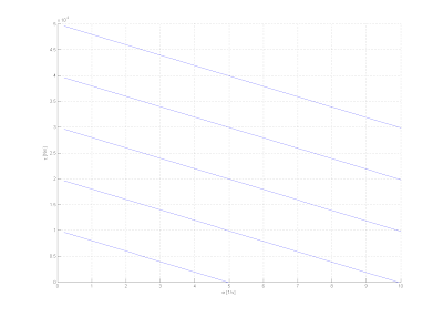
With this value we could draw tau - speed curves for various input voltages V_i.

6. Estimate the mechanical time constant of your motor. It will be related to your estimates of inertia and drag/damping.

The mechanical time constant of our motor remains as tau=1/delta=1.85.

7. Briefly describe what your velocity controller feels like when you turn the motor shaft. Why does it feel this way?

Position Feedback Simulation - Simulink Model:

Stepresponse in Theta:

2. Certainly include the results of your experimental and theoretical frequency response experiments. Both frequency response plotted on the same graph facilitates easy visual comparison and will be duly rewarded.

We built up a theoretical simulation of our motor with voltage as input and angular displacement Theta as output. The block diagram and the transfer function is shown below.

The bode diagram remains as follows. It shows a low amplification for high frequencies as we found it in our experiments in the same way.

In a next step we measured the angular displacement of the armature as a response to different input frequencies of voltage. We plotted the maximum output amplitude over the input frequencies.
The low conformity with the theoretical data is possibly due to the fact that measuring amplitudes with the hall effect sensor resulted difficult. In each experiment it is probable to observe at least one high amplitude to other generally lower amplitudes.

Sensors... So how do I know that you see the same blue as I see?

David Maiden Mueller

Colin Foe Parker

Yashar Ganjeh

Tim Stutz

Lab three is all about the glorious world of sensors, microprocessor integration, and even delving a little into the world of labView. We were given a Button, Pot, Photoresistor, Force Sensing Resistor, Photo interruptor, Hall Effect Sensor, LED's, a speaker, and a Hobby Servo and told to go to town. I mean, not literally town... because that is quite a walk.... but rather go play/build/tinker/learn. The end goal? Build a electronic musical instrument of some form that uses an Analog sensor for pitch and some other sensor for either articulation or volume. There were a few waypoints along the way.... 1. Read all the sensors as Digital Inputs in the Arduino. 2. Drive LED's off an Arduino GPIO. 3. Read Analog signals using the Arduino. 4. Run a Servo. 5. Play with LabView and try to do the same things again. So we weren't COMPLETELY unsupervised....

So, we met on Thursday all gungho and ready to start and build. Instead, we spent an hour and a half trying to rebuild what we had done the week before. As with all things... all four of us had built the previous weeks lab circuit differently. And everyone wanted to know WHY people chose which resistors or placed what parts where. So, we talked it out and eventually reached an amalgamation of different designs. Now it was time to actually start working on the lab. We went through the data sheets and laid out circuit diagrams for all the individual components. (Refer to Figures 1 through 3)

Figure 1: Circuit Layout

Figure 2: Circuit Layout

Figure 3: Circuit Layout

With this data, we were prepped to tackle sensor integration with the Arduino. We wrote a simple program that would take in sensor values. The system would the light up a LED if on. The code also saved the gpio value into the EEPROM and when all 512 memory locations were filled would dump the values onto the serial port. The code follows.

#include

int SensorPin = 52;

int LEDPIN = 13;

int Value;

int addr;

void setup(){

Serial.begin(9600);

pinMode(SensorPin,INPUT);

pinMode(LEDPIN,OUTPUT);

}

void loop(){

Value = digitalRead(SensorPin);

digitalWrite(LEDPIN,Value);

EEPROM.write(addr,Value);

if (addr == 512){

addr = 0;

while (addr <>

Value =EEPROM.read(addr);

Serial.println(Value, DEC);

addr = addr + 1;

}

addr = 0;

}

addr++;

delay(20);

}

This code worked for all digital pins. We then did the same test with an analog input. We used the same code with an exception of switching the "int SensorPin = 52;" to "int SensorPin = 0;" and the "Value= digitalRead(SensorPin)" to "Value = analogRead(SensorPin)'. As expected, the led did not light up unless the analog signal was truthfully 0. But all the rest of the components worked like a charm. :) The following graph shows the analog output of the arduino after 500 time steps.

Our next task was to get the servo up and running. The great thing about the arduino is that all the hard stuff is already done for us. We don't have to go through all the ports searching for the pwm output timers, or set up clocks to output at the right frequencies, or figure out how to scale the pwm duty cycle to get the servo running. Instead, all we have to do is "#include " set up a class and then tell the servo what to do. We got it up and running in <>

#include

#include

int SensorPin = 0;

int LEDPIN = 13;

int Value;

int addr;

Servo Servo1;

int i;

void setup(){

Serial.begin(9600);

Servo1.attach(12);

// pinMode(SensorPin,INPUT);

pinMode(LEDPIN,OUTPUT);

}

void loop(){

Value = analogRead(SensorPin);

digitalWrite(LEDPIN,Value);

EEPROM.write(addr,Value);

if (addr == 512){

addr = 0;

while (addr <>

Value =EEPROM.read(addr);

Serial.println(Value, DEC);

addr = addr + 1;

}

addr = 0;

}

addr++;

if (i > 5) {

Servo1.write(255);

}

else {

Servo1.write(0);

}

if (i==10){

i=0;

}

i++;

delay(100);

}

Our final task was to make a musical instrument of some form. We immediately decided make something that resembled a thermin. (I guess we aren't all that inventive...) However, we added a little twist. We would use the Hall Effect Sensor to control the pitch of the sound. We attached the Hall Effect sensor to an analog input of the Arduino. We would measure the value and using a gpio bitbang an output signal resembling a pwm. David devised a cool way to augment the signal to give it the traditional 8 bit Mario Kart video game sound that we all grew up with. The arduino output signal was then fed into a Nand gate in addition to an input from the photo interrupter. The result was fed into the NPN BJT and controlled a speaker output. The result? We developed a really cool electric instrument that augmented frequency by moving a magnet and controlled articulation with a blocker in the photo interrupter. Tim became pretty adept at making some hip tunes. Watch the embedded video below!!!

The code is following.....

const int sensorPin = 2; // pin that the sensor is attached to

const int ledPin = 22; // pin that the LED is attached to

const int outputOne = 24;

const int sensorGate = 52;

int outVal = 0; // value of the output

// variables:

int sensorValue = 0; // the sensor value

int sensorMin = 1023; // minimum sensor value

int sensorMax = 0; // maximum sensor value

int time = 1;

double frequency = 1;

void setup() {

pinMode(ledPin, OUTPUT);

pinMode(outputOne, OUTPUT);

pinMode(sensorGate, INPUT);

// turn on LED to signal the start of the calibration period:

pinMode(13, OUTPUT);

digitalWrite(13, HIGH);

// calibrate during the first five seconds

while (millis() <>

sensorValue = analogRead(sensorPin);

// record the maximum sensor value

if (sensorValue > sensorMax) {

sensorMax = sensorValue;

}

// record the minimum sensor value

if (sensorValue <>

sensorMin = sensorValue;

}

}

// signal the end of the calibration period

digitalWrite(13, LOW);

Serial.begin(9600);

}

void loop() {

// read the sensor:

sensorValue = analogRead(sensorPin);

// apply the calibration to the sensor reading

sensorValue = map(sensorValue, sensorMin, sensorMax, 0, 255);

// in case the sensor value is outside the range seen during calibration

sensorValue = constrain(sensorValue, 0, 255);

// fade the LED using the calibrated value:

//analogWrite(ledPin, sensorValue);

time = sensorValue*15;

//Serial.print("Sensor Value: ");

//Serial.print(sensorValue);

//Serial.print(" Time: ");

//Serial.print(time);

//Serial.print(" Frequency: ");

//Serial.println(frequency);

digitalWrite(outputOne, digitalRead(sensorGate));

for(int i=0; i<25;>

digitalWrite(ledPin, HIGH);

//outVal = digitalRead(ledPin);

//Serial.println(outVal);

delayMicroseconds(time);

digitalWrite(ledPin, LOW);

//outVal = digitalRead(ledPin);

//Serial.println(outVal);

delayMicroseconds(time);

}

}

The final aspect of our lab was to play with LabView.... After trying to figure out which computer actually had working DAQ's, what the difference was between a waveform graph and waveform chart, and what sampling frequency we wanted we were able to develop a while loop that sampled data the voltage out of a power supply and displayed it onto the computer screen. We added some buttons to light up software LED's and display funky stuff. All in all, the LabView part was just to get acquainted with the DAQ and the graphical programming layout.

So I guess thats all folks! Lab 3 was fun. And brought back good memories of nintendo games!